Data Visualization Exercises

If you and your group have any questions or get stuck as you work through this in-class exercise, please ask the instructor for assistance. Enjoy!

We are continuing to use the Global Superstore Orders 2016 Excel spreadsheet

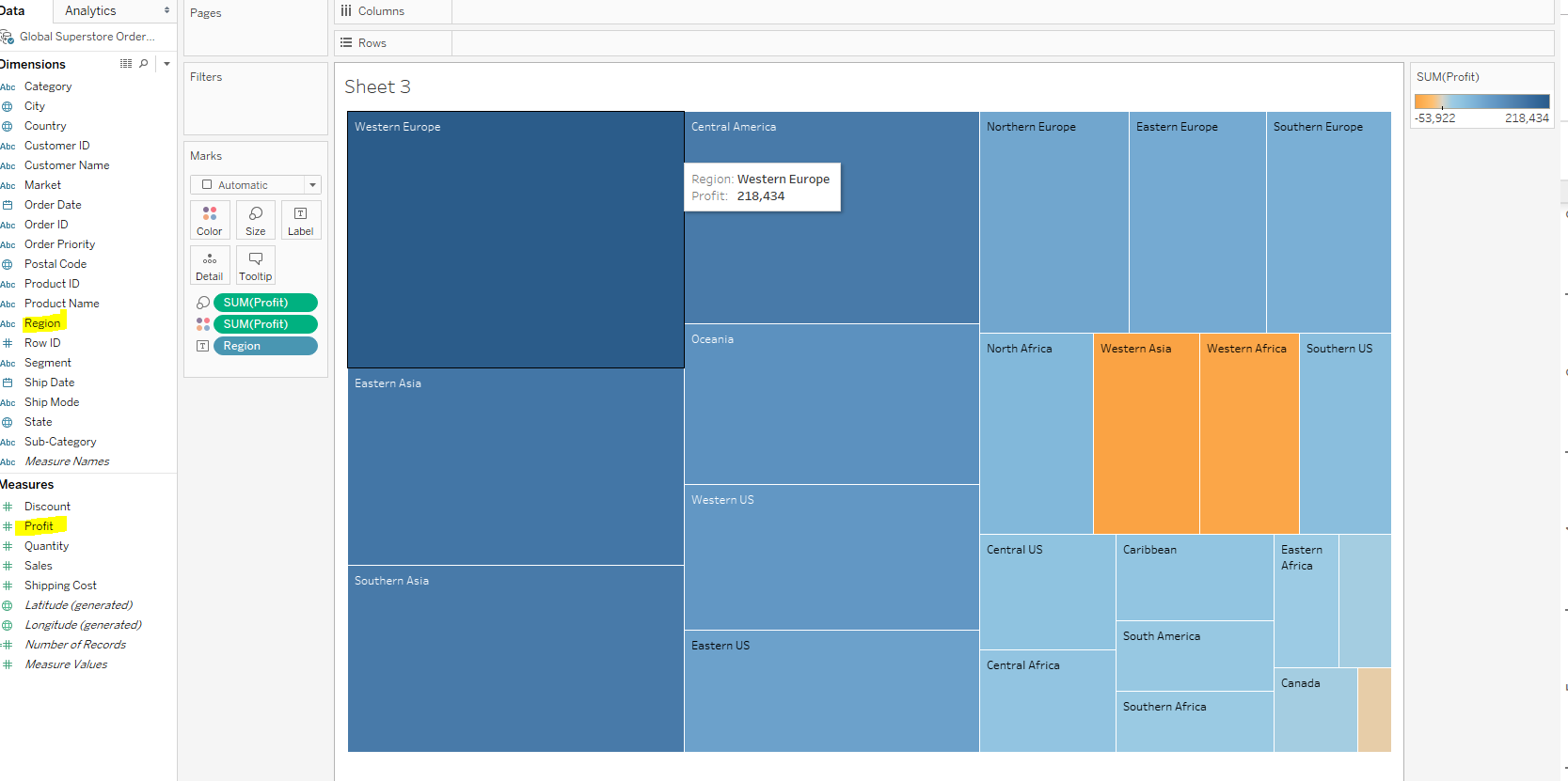
Treemap: Total Profit by Region
- Create a new sheet by clicking on the icon on the page-bottom menu
- From the dimensions list, right-click on Region and drag it up to the Rows shelf
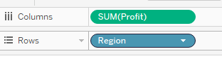
- From the measures list, right-click on Profit and drag it up to the Columns shelf. It will default to SUM(Profit) and a bar chart will display showing both negative and positive profits
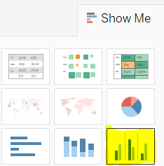
- Click on the Show Me icon in the top right corner of the screen to see the suggested visualizations
- Click on treemaps (4th one down on left)
- A grey pill stating 3 negative should appear at the bottom right corner. Click on this pill to view the two options for dealing with the negative values: Filter Data or Use Absolute Values
- By selecting Use Absolute Values, the negative values will appear as the same size as positive values but in a different colour
- Right-click Sheet 2 and rename it to Profit by Region Treemap. Automatically the data viz title changes to reflect the new name. Right-click the data viz title to edit further
- !! Remember if you make any mistakes, use the back arrow key at the top left of the top toolbar to go back !!

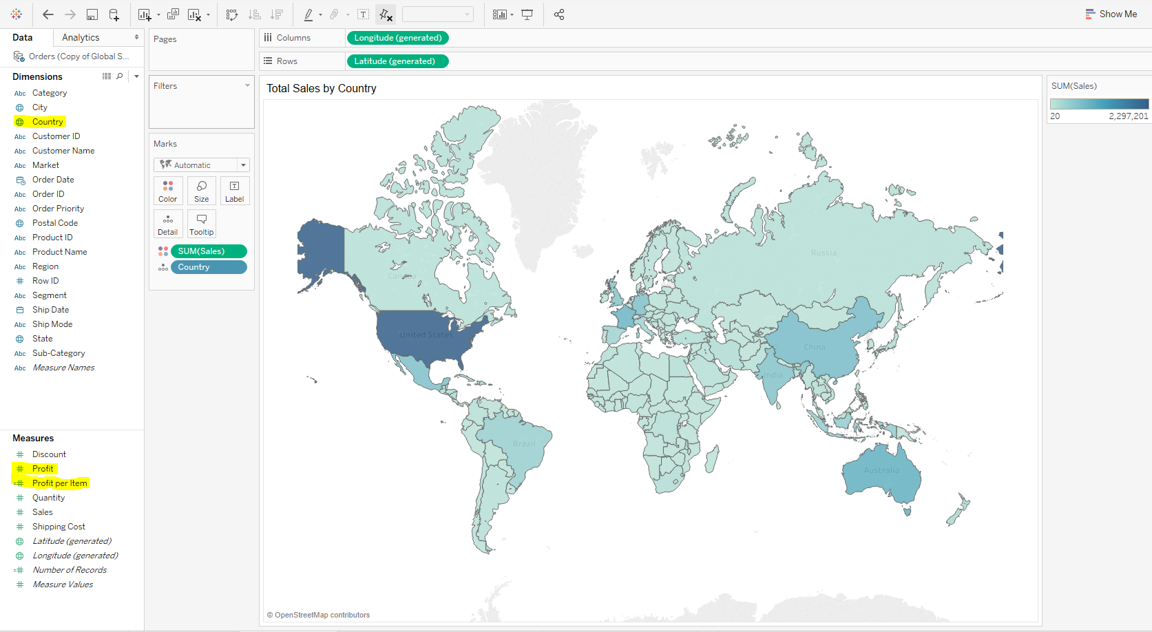
World Map: Total Sales by Country
- Create a new sheet by clicking on the icon on the page-bottom menu
- From the dimensions list, right-click and drag Country to the central drop field here area in the middle of the screen. Select Country from the dialogue box that appears
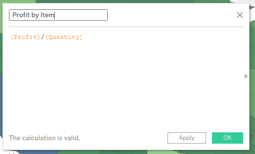
- To create a new measure, click Analysis on the top menu bar, and select Create Calculated Field from the drop-down menu (Note: For Mac users, the Analysis button will be in the very top Mac ribbon, not the Tableau app’s ribbon). In the pop-up text box, rename the default title Calculation1 to Profit per Item. The text box below allows formulas to be written, combining numerical operators and measures together. Left-click drag the Profit measure into the text box, type the division symbol ( / ), then left-click drag the Quantity measures, calculating profit per item

From the measures list, right-click and drag the new Profit per Item measure to the Color icon (see right) in the Marks box. Select AVG(Profit per Item). Now each country on the map will be colour-coded by the measure
To scroll around the world map, click on the black right-facing arrowhead in the zoom menu bar at the rop-left corner of the map, and select the crossed arrows. This will allow users to pan across the map
Let’s replace our calculated measure. Right-click the AVG(Profit per Item) green pill from the marks box and select remove

From the measures list, right-click on Sales and drag to the Color icon in the Marks box. Select SUM(Sales)
Edit map title and rename it Total Sales by Country
Try changing colors by clicking on Color in the Marks box and selecting Edit Colors

Line & Bar Chart (Dual Combo): Quarterly Profit and Number of Sales by Product 2012-2015
- Create a new sheet by clicking on the icon in the page-bottom menu
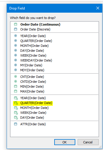
- From the dimensions list, right-click on Order Date and drag to the columns shelf. From the dialogue box that appears, select the QUARTER(Order Date) measure option (green w/ calendar & clock icon) (see figure ->). Note: this may not automatically appear for Mac users, so they must instead click on the ”+” next to YEAR(Order Date)
- From the measures list, right-click on Sales and drag to the rows shelf. Select CNT(Sales) from the pop-up box
- Again, from the measures list, right-click on Profit and drag to the rows shelf, then select SUM(Profit)
- From the dimensions list, right-click on Category and drag to the rows shelf

Click the Show Me icon (top-right) and select the dual combination chart (3rd up from the bottom right). Click again on the Show Me icon again to close it
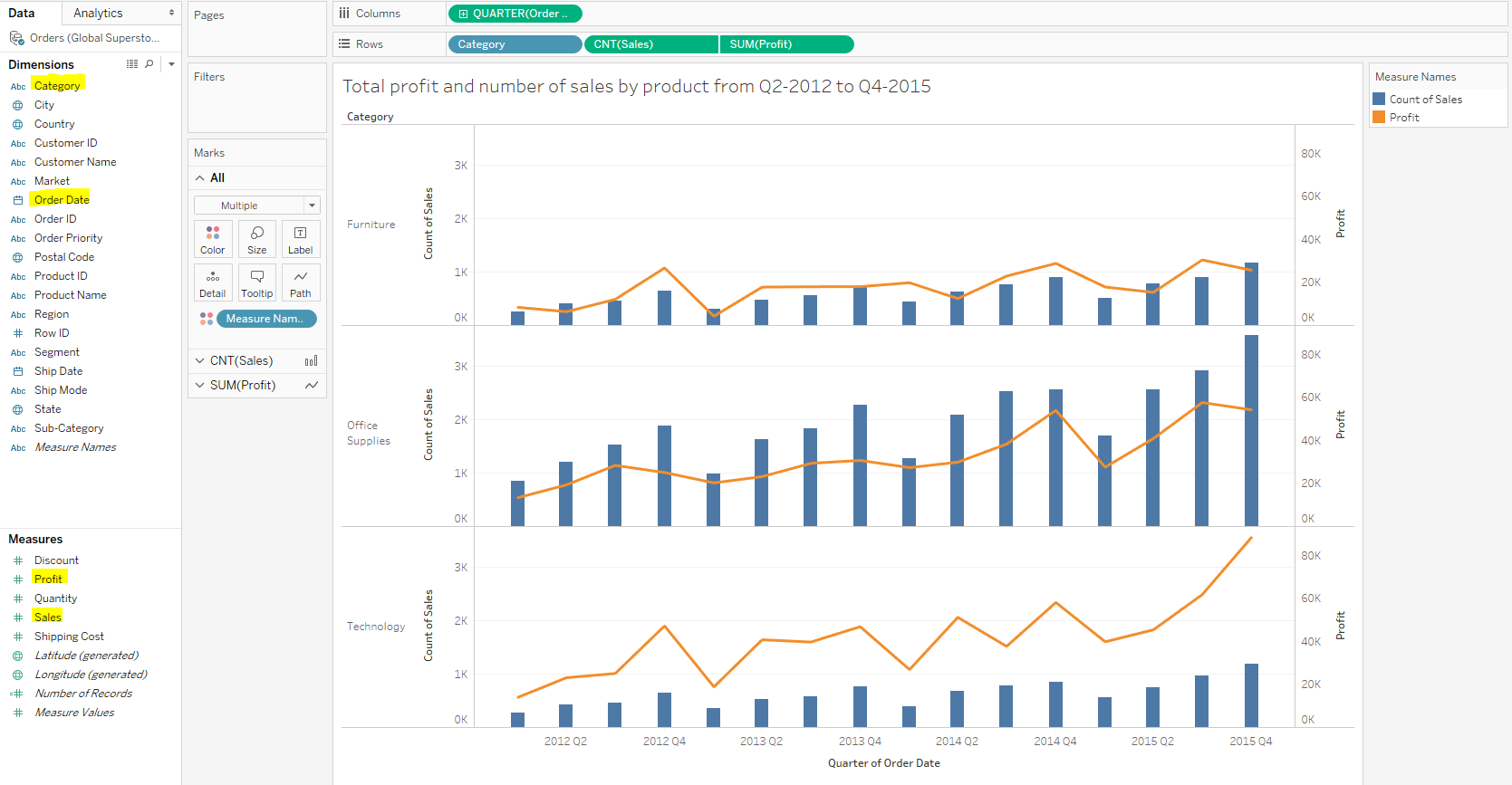
Rename the title to Quarterly Profit and Sales by Product

Building Sales Graphs for the Interactive Dashboard
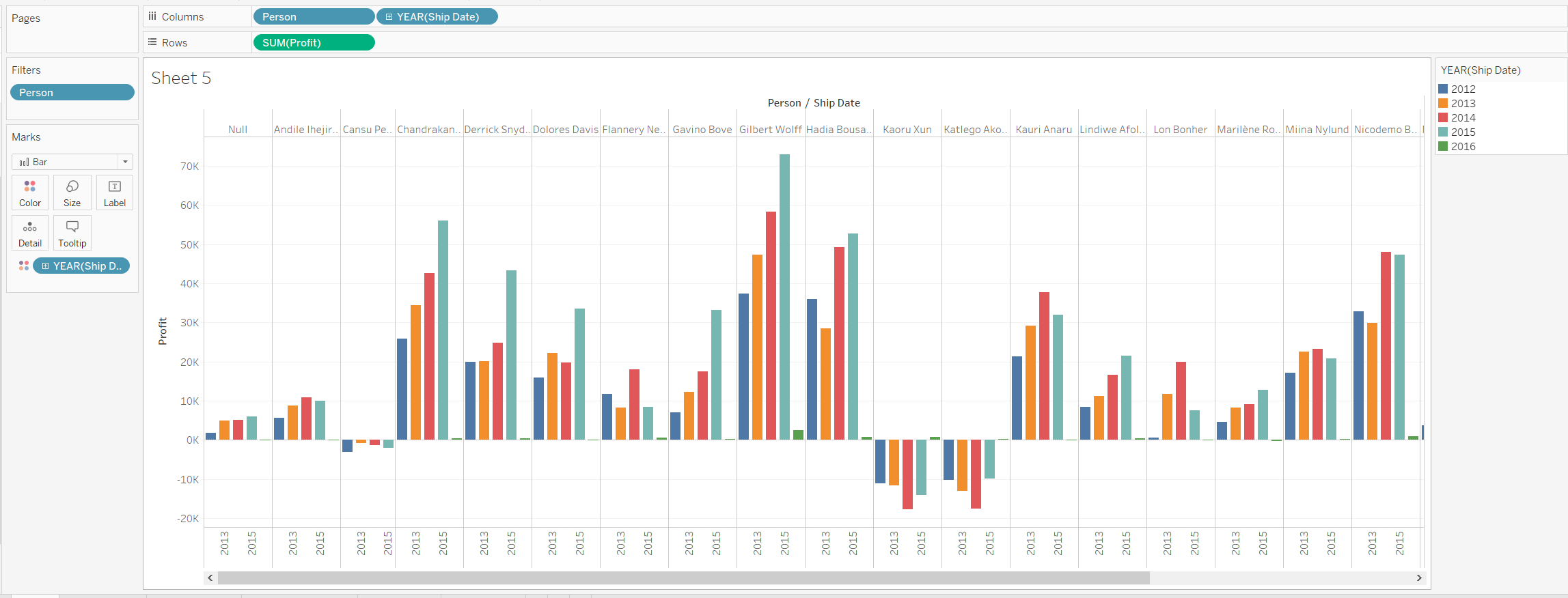
- Profit by Year Graph
  1. Return to Data Source and drag the People sheet to the same area as Orders
  2. Click on the New Worksheet tab at the bottom of the graph from the tables menu, click and drag Person to the Columns
  1. Click on Ship Date and drag it to the Columns as well
  2. Click on Profit and drag it to the Rows. It will automatically produce SUM(Profit)
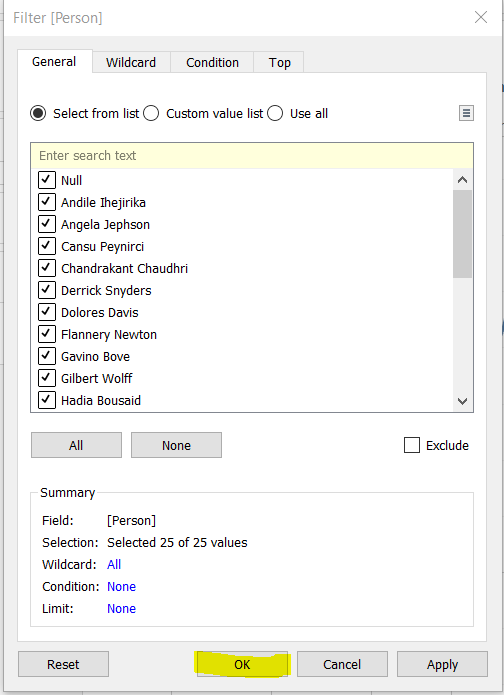
  3. From the Tables, grab Person and drag it into the Filters section and click OK in the pop-up window. This will allow us to filter the graph by a specific person
  4. From the Tables, grab Ship Date and drag it into the Color section in the Marks pane
  5. The last step is to click on Show Me icon in the top-right corner and select the Side-by-Side Bars option. After that, right-click on the name of your table at the bottom of the pane and rename it Profit by Year

Your final result should look like this:
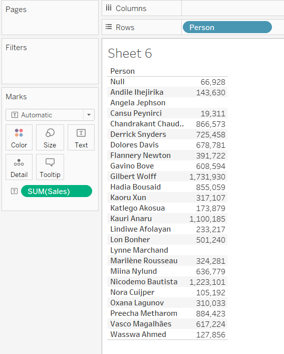
- Orders by Person Graph
  1. Click on the New Worksheet tab at the bottom of the graph
  2. From the Tables select Person and drag it onto Rows
  3. From the Tables select Sales and drag it onto Text in the Marks bar. The goal here is to show the numeric value without any calculations (Tableau will automatically convert the numbers to SUM)
  4. Right-click on your Sheet name at the bottom of the pane and rename it Orders by Person
  5. Your end result should look like this:
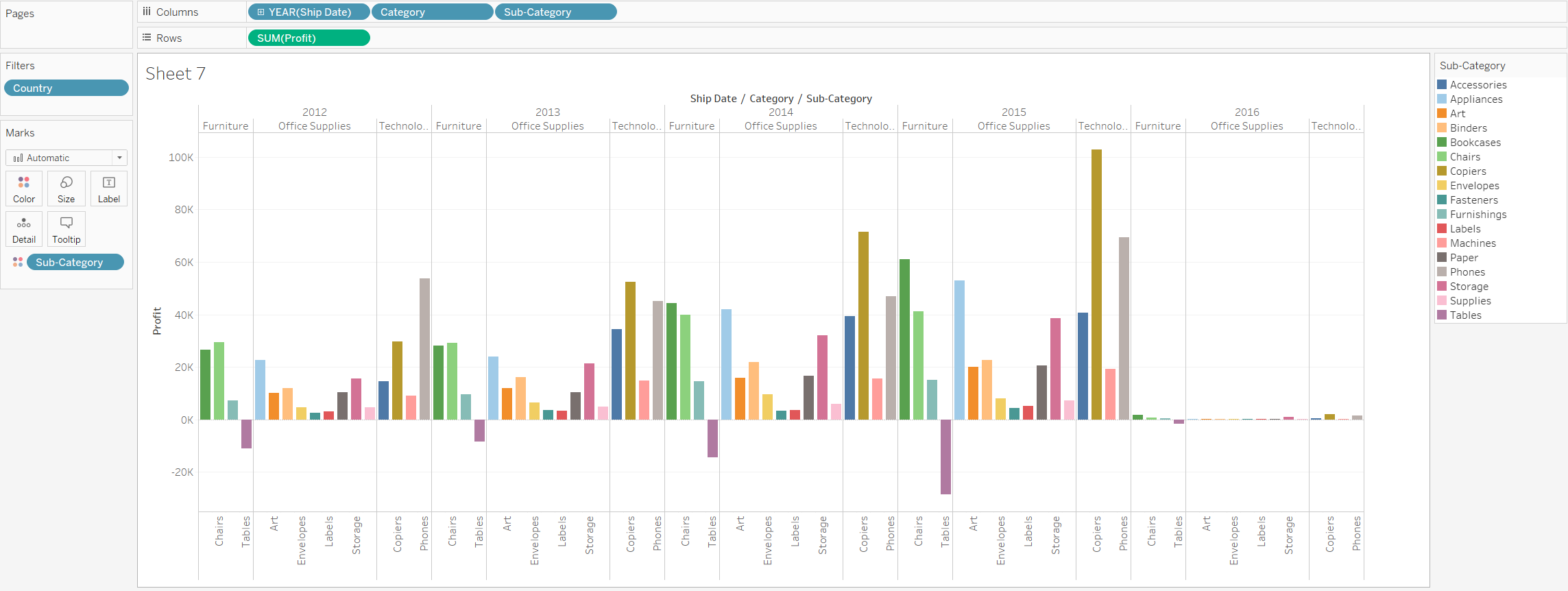
- Date/Category/Profit Graph
  1. Click on the New Worksheet tab at the bottom of the graph
  2. Click and drag Ship Date, Category and Sub-Category into the Columns
  3. Click and drag Profit into Rows
  4. Your Columns and Rows should look like this:
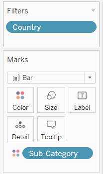
  5. Click and drag Sub-Category onto the Color pane in the Marks section
  6. Click and drag Country into the Filters section. In the pop-up window click All and click OK
  7. Rename your table “Date/Category/Profit”
  8. Your graph should look like this: