Linear regressions
Tips before you start:
-
You can pull up documentation for a function by executing
?function_name(e.g.?t.test) in the Console. -
You might want to start a new .Rmd file for this activity
-
Throughout this workshop, instead of typing in commands directly in the command line or in the code editor, type them in chunks of code in your .Rmd file.
-
Now that you are bit more familiar on how to use .Rmd files,there are some additional tips that make it using .Rmd files easier:
- You can run each individual chunk of code all at once by clicking on the little green arrow facing right at the top right of each chunk:

- You can run all chunks of code above by clicking on the little gray arrow facing down at the top right of each chunk:

- You can decide if you want R Studio to output the results of each chunk of code inline in your R Markdown file, or in the console. This is just for when your are actively working on the file, when knitting, all outputs appear right after the chunk of code. To decide, click on the setting buton on the right of the knitting button, and select the option you prefer.
- You can run each individual chunk of code all at once by clicking on the little green arrow facing right at the top right of each chunk:
-
Finally, have the tidyverse package installed and loaded in RStudio before you start this activity:
# only need to run once in the console if tidyverse not installed: install.packages('tidyverse')
library(tidyverse)
- If you need a reminder on data manipulation functions, check out the dplyr cheat sheet
Download data
In this activity, we will build linear models to predict life expectancy with one or more independent/explanatory variables. Download the Life Expectancy dataset by right clicking on this text and select “Download linked file as”. Save it in the same folder as your current R Markdown file.
The source of this data is this website.
Import the data
Import the dataset by typing the following in a code chunk, and then sending it to the command line:
# Import data
life_expectancy <- read.csv("WHO_Life_Expectancy_Data.csv") # change to the appropriate file path to the downloaded dataset on your computer
Let’s then preview the data to see if it was uploaded correctly (paste the code below in a chunk of code and then send it to the command line). As you can see, the data shows multiple variables possibly related to overall life expectancy for different countries over the years.
head(life_expectancy)
##       Country Year     Status Life.expectancy Adult.Mortality infant.deaths
## 1 Afghanistan 2015 Developing            65.0             263            62
## 2 Afghanistan 2014 Developing            59.9             271            64
## 3 Afghanistan 2013 Developing            59.9             268            66
## 4 Afghanistan 2012 Developing            59.5             272            69
## 5 Afghanistan 2011 Developing            59.2             275            71
## 6 Afghanistan 2010 Developing            58.8             279            74
##   Alcohol percentage.expenditure Hepatitis.B Measles  BMI under.five.deaths
## 1    0.01              71.279624          65    1154 19.1                83
## 2    0.01              73.523582          62     492 18.6                86
## 3    0.01              73.219243          64     430 18.1                89
## 4    0.01              78.184215          67    2787 17.6                93
## 5    0.01               7.097109          68    3013 17.2                97
## 6    0.01              79.679367          66    1989 16.7               102
##   Polio Total.expenditure Diphtheria HIV.AIDS       GDP Population
## 1     6              8.16         65      0.1 584.25921   33736494
## 2    58              8.18         62      0.1 612.69651     327582
## 3    62              8.13         64      0.1 631.74498   31731688
## 4    67              8.52         67      0.1 669.95900    3696958
## 5    68              7.87         68      0.1  63.53723    2978599
## 6    66              9.20         66      0.1 553.32894    2883167
##   thinness..1.19.years thinness.5.9.years Income.composition.of.resources
## 1                 17.2               17.3                           0.479
## 2                 17.5               17.5                           0.476
## 3                 17.7               17.7                           0.470
## 4                 17.9               18.0                           0.463
## 5                 18.2               18.2                           0.454
## 6                 18.4               18.4                           0.448
##   Schooling
## 1      10.1
## 2      10.0
## 3       9.9
## 4       9.8
## 5       9.5
## 6       9.2
Prepare the data
We are going to use only data from the year of 2015 as it is most recent. For this, use the filter()function from dplyr (i.e.g, part of the tidyverse package), which we cover in the workshop Introduction to RStudio. Paste the code below in a chunk of code and then send it to the command line:
# Filter the dataset
life_expectancy_2015 <- life_expectancy %>%
  filter(Year == 2015)

# Check results
head(life_expectancy_2015)
##               Country Year     Status Life.expectancy Adult.Mortality
## 1         Afghanistan 2015 Developing            65.0             263
## 2             Albania 2015 Developing            77.8              74
## 3             Algeria 2015 Developing            75.6              19
## 4              Angola 2015 Developing            52.4             335
## 5 Antigua and Barbuda 2015 Developing            76.4              13
## 6           Argentina 2015 Developing            76.3             116
##   infant.deaths Alcohol percentage.expenditure Hepatitis.B Measles  BMI
## 1            62    0.01               71.27962          65    1154 19.1
## 2             0    4.60              364.97523          99       0 58.0
## 3            21      NA                0.00000          95      63 59.5
## 4            66      NA                0.00000          64     118 23.3
## 5             0      NA                0.00000          99       0 47.7
## 6             8      NA                0.00000          94       0 62.8
##   under.five.deaths Polio Total.expenditure Diphtheria HIV.AIDS        GDP
## 1                83     6              8.16         65      0.1   584.2592
## 2                 0    99              6.00         99      0.1  3954.2278
## 3                24    95                NA         95      0.1  4132.7629
## 4                98     7                NA         64      1.9  3695.7937
## 5                 0    86                NA         99      0.2 13566.9541
## 6                 9    93                NA         94      0.1 13467.1236
##   Population thinness..1.19.years thinness.5.9.years
## 1   33736494                 17.2               17.3
## 2      28873                  1.2                1.3
## 3   39871528                  6.0                5.8
## 4    2785935                  8.3                8.2
## 5         NA                  3.3                3.3
## 6   43417765                  1.0                0.9
##   Income.composition.of.resources Schooling
## 1                           0.479      10.1
## 2                           0.762      14.2
## 3                           0.743      14.4
## 4                           0.531      11.4
## 5                           0.784      13.9
## 6                           0.826      17.3
Simple linear regression
Linear regressions are used when we want to investigate relationships between variables. For example, in this case, imagine we want to investigate if overall life expectancy is related to the level of schooling of the country. This is different than in the previous activity, when we wanted to test if different groups had different means.
The lm() command creates a linear regression model. It takes the following format:
lm(response_variable ~ predictor_variables, data = data_source)
In this case, life expectancy is our response variable (i.e., we expect it to respond to the level of schooling), and schooling is our predictor variable (i.e., we expect it to predict life expectancy).
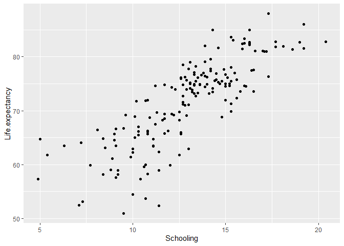
Visualize trends
To start, you first want to visualize the relationship in a plot to see if a linear relationship is reasonable. We will be using ggplot (part of the tidyverse package) to plot throughout this workshop. This was covered in the workshop Introduction to RStudio:
Type this in a code chunk and then send it to the command line:
# Create a scatter plot of life expectancy by Schooling
ggplot(data = life_expectancy_2015, # specify the data
       aes(x = Schooling, y = Life.expectancy)) + # specify the variables
  geom_point() # plot a scatter plot
Fit a simple linear regression
The plot shows that a linear relationship is reasonable. Therefore, we will create a simple linear regression model where the response variable is Life expectancy and the predictor variable is Schooling. The model can be written as:
life expectancy = intercept + slope * schooling
In R, type this in a code chunk and send it to the command line:
# Fit the model
lm_schooling <- lm(Life.expectancy ~ Schooling, data = life_expectancy_2015)

# See the results of the model
summary(lm_schooling)
##
## Call:
## lm(formula = Life.expectancy ~ Schooling, data = life_expectancy_2015)
##
## Residuals:
##     Min      1Q  Median      3Q     Max
## -15.909  -2.547   0.317   3.170  10.655
##
## Coefficients:
##             Estimate Std. Error t value Pr(>|t|)
## (Intercept)  42.9016     1.5870   27.03   <2e-16 ***
## Schooling     2.2287     0.1198   18.61   <2e-16 ***
## ---
## Signif. codes:  0 '***' 0.001 '**' 0.01 '*' 0.05 '.' 0.1 ' ' 1
##
## Residual standard error: 4.575 on 171 degrees of freedom
##   (10 observations deleted due to missingness)
## Multiple R-squared:  0.6694, Adjusted R-squared:  0.6675
## F-statistic: 346.2 on 1 and 171 DF,  p-value: < 2.2e-16
There is a lot of information in this output:
-
Call: a reminder of the model you just fitted.
-
Residuals: a summary of the distribution of the residuals of the model. The residuals are the difference between the observed values and the value predicted by the model. You want this distribution to be normal, and comparing these values can help you inspect that, however, you will typically inspect this in other ways (see topic on assumptions below).
-
Coefficients: this is the main result of the model. It shows you the estimated values for the intercept and the slope (i.e., the slope for Schooling, in this case), the standard error of these estimates (i.e., the uncertainty around these estimates), and the results of a t-test (the t-value and the p-value associated with it) testing whether these values are significantly different from 0.
-
The small p-values for the coefficients (<0.001) indicate that the estimates for the intercept and slope are statistically significant. The specific values mean that we can write the model mathematically as: Life expectancy = 42.9016 + 2.2287 * Schooling.
-
The bottom part of the results gives you a summary of the overall fit of the model (i.e., how well the model explains your data). The most important are the R-squared, which tells you how much variance the model explains, and the results associated with the F-statistic, which tells you the significance of your entire model (and not just each individual coefficients, as the t-tests above show).
-
In this case, the R-squared value of 0.6694 indicates that 66.94% of the variance in Life Expectancy is explained by Schooling. The high R-square and the small p-value here (<0.001) tell you that this model is a good fit that explains a lot of variance in your data.
You might also want to get the 95% confidence interval for the coefficient estimates. Type this in a chunk of code and send it to the command line:
# Get confidence intervals of model estimates
confint(lm_schooling)
##                2.5 %    97.5 %
## (Intercept) 39.76897 46.034216
## Schooling    1.99229  2.465164
We can also visualize this model by adding a regression line to the plot. For that, type this in a chunk of code and send it to the command line:
# Create a scatter plot of life expectancy by Schooling with the fitted line of a linear regression
ggplot(data = life_expectancy_2015, # specify the data
       aes(x = Schooling, y = Life.expectancy)) + # specify the variables
  geom_point() + # plot a scatter plot
  geom_smooth(method = "lm") # add a fitted line with confidence intervals using the linear model (lm) method
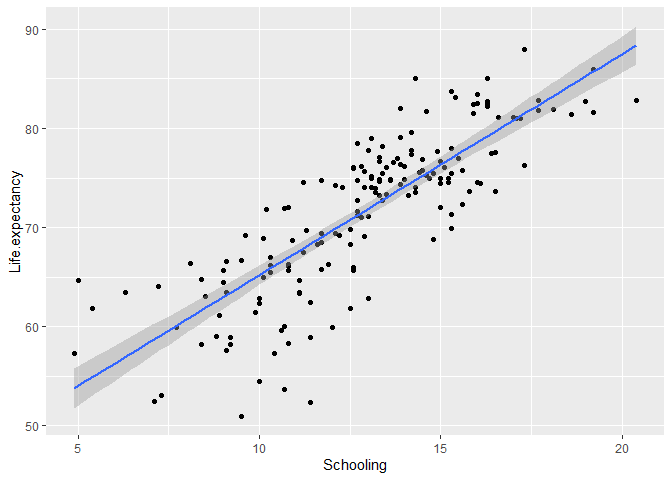
It seems like the line explains the trend in the data well. However, you will still want to check if the model meets the assumptions before you make any inferences from this model.
Assumptions
Linear regression makes several assumptions about the data, which form the acronym LINE: linearity, independence, normality, and equal variance of the residuals. To inspect these assumptions, you can use the function plot() on a lm object in R (i.e. the object with results of a linear model), which plots 4 useful diagnostics plots for regression models.
- Linearity: the model assumes the relationship between the variables is a linear relationship. You can check that visually in the scatter plot above. Another way to inspect is to plot the residuals of the model as a function of the fitted values (paste the code below in a chunk of code and then send it to the command line). If the relationship is linear, the line should be flat (i.e., observations are equally distributed above and below the line of fitted values of a linear model).
# Plot residuals versus fitted values
plot(lm_schooling, 1) # the number 1 tells R to plot the 1st diagnostic plot
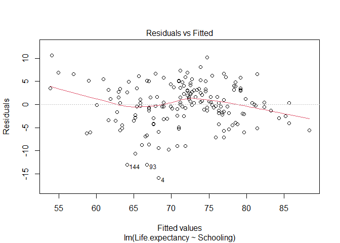
The line is not perfectly flat, but it is reasonably close. Still, it suggests it might be good to examine the points with small and large fitted values as they seem to be the ones deviating from the flat line.
-
Independence: the model assumes each observation is independent of the others. Although there are ways to visually inspect this assumption if you have concerns about temporal or spatial non-independence, as we have seen in the previous section, usually this assumption is met by considering the structure of the data. In this case, we can reasonably assume that the countries are independent observations.
-
Normality of the residuals: the model assumes the residuals are normally distributed. To inspect this, you can check a Q-Q Plot of the residuals (paste the code below in a chunk of code and then send it to the command line). In this plot, the points should be close to the line (i.e. the line shows what would be expected for a normal distribution).
# Plot Q-Q plot of the residuals
plot(lm_schooling, 2) # the number 2 tells R to plot the 2nd diagnostic plot
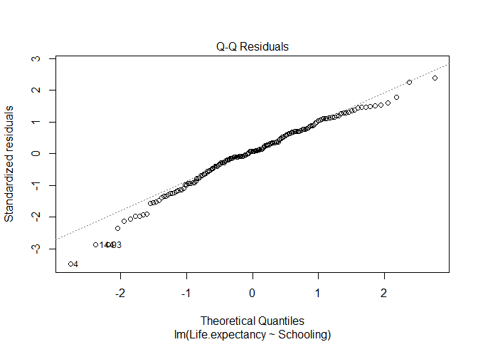
Again, overal the points are close to the line, but there seem to be a few outliers. We may want to examine these data points in further analysis.
- Equal variance of the residuals: the model assumes the spread of the residuals around the fitted line (i.e. their variance) is the same for the entire range of the predictor variable. To inspect that, you can plot a scatter plot of standardized residuals versus fitted values (paste the code below in a chunk of code and then send it to the command line). Mainly, you want to check if this plot has a flat line, which would tell you the residuals have the same variance across the model.
# Plot Q-Q plot of the residuals
plot(lm_schooling, 3) # the number 3 tells R to plot the 3rd diagnostic plot
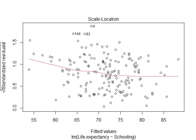
Again, the model seems to meet the assumption with a few outliers that might need to be examined further.
Multiple linear regression
Multiple linear regressions are very similar to simple regressions, but they contain more than one predictor variables. For example, we might want to expand our model to consider the simultaneous effect of schooling and an additional predictor variable, the average body mass index of the population (BMI).
Visualize trends
First, let’s visualize the relationships. Type the code below in a chunk of code and then send it to the command line.
life_expectancy_2015 %>%
  # Select the three relevant variables
  select(Life.expectancy, BMI, Schooling) %>%
  # plot pairwise correlation plots
  pairs()
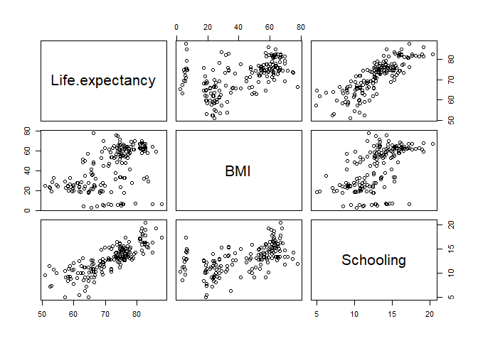
From the plot, BMI does not look as good as Schooling as a predictor of Life expectancy. But we will go ahead and fit a multiple regression model to have a concrete result.
Fit a multiple linear regression model
Create a multiple linear regression model where the response variable is Life expectancy and the predictor variables are BMI and Schooling. The model can be written as:
Life expectancy = slope_1 * BMI + slope_2 * Schooling + intercept
Type the following code in a chunk of code and send it to the command line to fit that model:
# Fit a multiple regression linear model
lm_multiple <- lm(Life.expectancy ~ Schooling + BMI, data = life_expectancy_2015)

# See the results of the model
summary(lm_multiple)
##
## Call:
## lm(formula = Life.expectancy ~ Schooling + BMI, data = life_expectancy_2015)
##
## Residuals:
##      Min       1Q   Median       3Q      Max
## -15.4768  -2.4894   0.1514   3.0108  11.2459
##
## Coefficients:
##             Estimate Std. Error t value Pr(>|t|)
## (Intercept) 42.57196    1.66503  25.568   <2e-16 ***
## Schooling    2.16981    0.15029  14.437   <2e-16 ***
## BMI          0.02442    0.02045   1.194    0.234
## ---
## Signif. codes:  0 '***' 0.001 '**' 0.01 '*' 0.05 '.' 0.1 ' ' 1
##
## Residual standard error: 4.569 on 168 degrees of freedom
##   (12 observations deleted due to missingness)
## Multiple R-squared:  0.6677, Adjusted R-squared:  0.6638
## F-statistic: 168.8 on 2 and 168 DF,  p-value: < 2.2e-16
As we thought, BMI is not a significant predictor variable with a p-value of 0.234. The model is still significant however, with p-value of 2.2e^-16, because Schooling is included. We conclude that the simple regression model adequately fits the data. For the sake of completeness, the multiple regression model can be written as:
Life expectancy = 2.16981 * Schooling + 0.02442 * BMI + 42.57196
Assumptions
Similar to the simple model, this command produces graphs to check the model assumptions. Type the code below in a chunk of code and then send it to the command line.
# Changes plotting setting to create a panel with two rows and two columns to plot 4 graphs
par(mfrow = c(2,2))

# Plot the diagnostic plots (without number, R will plot all four plots)
plot(lm_multiple)
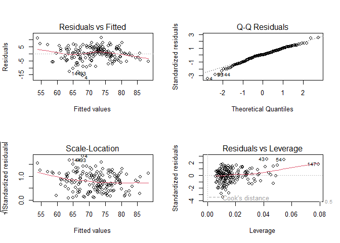
# Returns the settings for plots for single plot (one row and one column)
par(mfrow = c(1,1))
Again, the model does not seem to deviate much from assumtpions, but some outliers might be worth investigating further. The Residuals vs Leverage plot is helpful to identify outliers that might be affecting the model: they are shown with the number of observation right next to (i.e., in this case, observations number 43, 54, and 147 are outliers)
Conduct a single or multiple regression analysis with other variables of your choosing
You can now use the life_expectancy dataset to explore other relationships of your choosing. For that:
- Make a scatter plot to explore their linear relationship
- Build a linear regression model
- Assess the results. Let the instructors know if you need help!
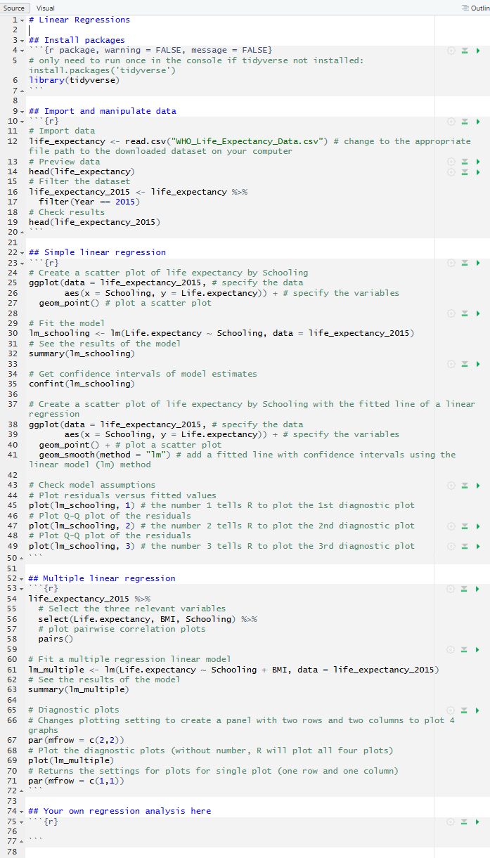
As the end of this activity, your Markdown file may look like this:
Again, knit this document into a .pdf and see how it looks!