Test for Difference in Means (t-tests, ANOVA)
Tips before you start:
-
You can pull up documentation for a function by executing
?function_name(e.g.?t.test) in the Console. -
Also, a quick note…
A quick note about using AI
As you work through this workshop, you may feel tempted to ask an AI model for help with the exercises. We discourage this because delegating something to AI can prevent you from developing that skill. In fact, one of the most effective ways to learn R is to troubleshoot code by yourself. AI models can also hallucinate and produce incorrect code, so you need to understand enough about R to be able to evaluate their output. If AI is doing all your coding for you and you don’t learn the underlying logic and syntax of R, it will be harder for you to verify their output. Remember, you should think of AI as your research assistant, and you are still responsible for any code produced by AI. Also note that, if you want an AI model to develop code for your data, you should be careful about sharing confidential information (i.e. your dataset) with AI models, and should only do so if you have ethics approval. That being said, AI can definitely be a helpful tool, especially if you use with the right attitude and know what and how to ask for the most useful responses. While this workshop doesn’t cover best practices for using AI in coding, you can find some useful tips here and here.
Organize your .Rmd file
Before we start, clean the content of your markdown file:
-
Delete all the example text and chunks of code that came with it when you opened the template.
-
Give a heading for this activity by typing
# Activity 2at the top -
Start a second-level heading for the one sample t-test below by typing
## One-sample t-testin the line below -
Create a chunk of R code. You can do this in multiple ways:
- Type in “```{r}” in one line, hit enter twice, and type in “```” to finish the code chunk.
- Click on the “Insert a new code chunk” button at the top right, and then select R:
- Use the keyboard shortcut “Ctrl + Shift + I” (for windows)
Now you can start going through the workshop activities! Throughout this workshop, instead of typing in commands directly in the command line or in the code editor, type them in the chunks of code in your .Rmd file.
One-sample t-test
One-sample t-test is a hypothesis test to see whether the mean of a dataset is significantly different from a value.
As an example, we have test scores for a sample of 10 students. The scores are 75, 91, 68, 83, 66, 94, 85, 86, 75, and 80. We use a one-sample t-test to see if the sample mean is significantly different from 65 at the 0.05 level. The null hypothesis is that μ = 65 (μ is a character usually used to indicate population mean).
In the Code Editor (inside a chunk of code in your RMarkdown file), create a data vector called scores, and then click Ctrl + Enter (PC) or Cmd + Enter (Mac) to run the code in the command line.
# Create the vector with score values
score <- c(75, 91, 68, 83, 66, 94, 85, 86, 75, 80)
Conduct a one-sample t-test and report the t-statistic and p-value. By default, the test performs a two-sided test, which means the alternative hypothesis is that μ is different from 65. Add to the code chunk in your RMarkdown file, and then send to the command line:
# Perform a one-sample t-test to test if the mean of the sample is different than 65
t.test(score, mu = 65)
##
##  One Sample t-test
##
## data:  score
## t = 5.2102, df = 9, p-value = 0.0005564
## alternative hypothesis: true mean is not equal to 65
## 95 percent confidence interval:
##  73.65706 86.94294
## sample estimates:
## mean of x
##      80.3
The p-value is smaller than 0.05, so we would reject the null hypothesis and conclude that the population mean is significantly different from 65.
You can also test a directional hypothesis, for example if the alternative hypothesis is that the population mean is greater than 65 at the .05 level. To do that, you need to specify the alternative argument in the t.test() function. The parameter of this argument must be one of the following: "two.sided" (which is the default), "greater", or "less", depending on whether the alternative hypothesis is that the mean is different than, greater than or less than μ, respectively.
Therefore, to test if the population mean is greater than 65, add the following in a code chunk in your RMarkdown file, and then send to the command line:
# Perform a one-sample t-test to test if the mean of the sample is greater than 65
t.test(score, mu = 65, alternative = "greater")
##
##  One Sample t-test
##
## data:  score
## t = 5.2102, df = 9, p-value = 0.0002782
## alternative hypothesis: true mean is greater than 65
## 95 percent confidence interval:
##  74.91697      Inf
## sample estimates:
## mean of x
##      80.3
The p-value is smaller than 0.05, so we reject the null hypothesis and conclude that the population mean is significantly greater than 65.
⭐ Task 2-1
Test another alternative hypothesis
Try conducting a one-sample t-test where the alternative hypothesis is the mean is less than 65. What is the R command and what is your conclusion?
Check the answer
# Perform a one-sample t-test to test if the mean of the sample is less than 65
t.test(score, mu = 65, alternative = "less")
##
##  One Sample t-test
##
## data:  score
## t = 5.2102, df = 9, p-value = 0.9997
## alternative hypothesis: true mean is less than 65
## 95 percent confidence interval:
##      -Inf 85.68303
## sample estimates:
## mean of x
##      80.3
With a p-value larger than 0.05, we cannot reject the null hypothesis that the population mean is equal to or higher than 65.
Assumptions
One-sample t-tests have two assumptions that you should check before making any inferences from your test:
-
The data is normally distributed.
-
There are no outliers in your data.
-
Additionally, the test also assumes the observations are independent from one another, but this is something that can not be tested or checked, but rather considered from the way the data is collected. In this case, we can reasonably assume that the score of each student is independent from one another.
To test if your data is normally distributed, you can perform a Shapiro-Wilk test. Type this in a chunk of code and then send it to the console:
# Performs a Shapiro-Wilk test to assess normality
shapiro.test(score)
##
##  Shapiro-Wilk normality test
##
## data:  score
## W = 0.96286, p-value = 0.8179
P-values smaller than 0.05 indicate that your data has low probability of arising from a normal distribution. In this case, because the p-value > 0.05, we can assume that our data comes from a normal distribution.
There are many methods to assess outliers, but a simple and quick way is to plot a boxplot (type in the code below and then send it to the command line. By default, boxplots show outliers as asterisks outside the range delimited by the whiskers. Type this code in a chunk of code and then send it to the console:
# Plot a box plot of the data
boxplot(score)
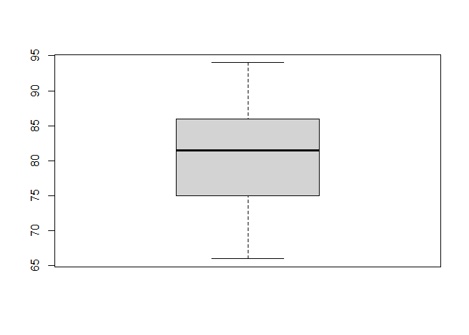
As you can see, there does not seem to be any outliers in our data.
Two-sample t-test
A two-sample t-test is a hypothesis test to see whether there is a significant difference between the means of two samples.
Consider two pizza companies, A and B. We want to test if there is a significant difference in the average pizza delivery times between A and B. Following are the data collected from a sample of delivery times (in minutes). μA = μB is the null hypothesis
| Delivery Time A | Delivery Time B |
|---|---|
| 25.4 | 25.2 |
| 29.2 | 21.9 |
| 22.4 | 23.5 |
| 26.4 | 22.3 |
| 25.2 | 25.5 |
| 23.5 | 23.6 |
| 26.5 | 22.3 |
Create two vectors for the delivery time of company A and company B in a code chunk in your RMarkdown file, and then send it to the command line.
# Create vectors with delivery times
companyA <- c(25.4, 29.2, 22.4, 26.4, 25.2, 23.5, 26.5)
companyB <- c(25.2, 21.9, 23.5, 22.3, 25.5, 23.6, 22.3)
Conduct a two-sample t test and report the t and p values by adding the following in a code chunk in your RMarkdown file, and then sending it to the command line:
# Performs two-sample t-test to test for difference in means
t.test(companyA, companyB)
##
##  Welch Two Sample t-test
##
## data:  companyA and companyB
## t = 2.0541, df = 10.301, p-value = 0.06624
## alternative hypothesis: true difference in means is not equal to 0
## 95 percent confidence interval:
##  -0.1643905  4.2501047
## sample estimates:
## mean of x mean of y
##  25.51429  23.47143
From the output, we can see that the p-value is 0.06624 > 0.05. Hence, there is no strong evidence showing a difference in the average times to deliver a pizza between Company A and Company B.
In the same way as for the one-sample t-test, you can specify different alternative hypothesis in the argument alternative.
⭐ Task 2-2
Test another alternative hypothesis
Try conducting a two-sample t-test where the alternative hypothesis is Company A delivers pizzas faster than Company B. What is the R command and what’s your conclusion?
Check the answer
# Perform a two-sample t-test to test if the mean of the sample of group 1 (company A) is smaller (i.e. faster) than group 2 (company B)
t.test(companyA, companyB, alternative = "less")
##
##  Welch Two Sample t-test
##
## data:  companyA and companyB
## t = 2.0541, df = 10.301, p-value = 0.9669
## alternative hypothesis: true difference in means is less than 0
## 95 percent confidence interval:
##      -Inf 3.840106
## sample estimates:
## mean of x mean of y
##  25.51429  23.47143
With a p-value larger than 0.05, we cannot reject the null hypothesis that the mean delivery time for company A is equal to or larger (i.e. slower) than the delivery time for company B.
Assumptions
The two-sample t-test also has assumptions that must be met before you can use the result to interpret your data. They are:
-
The two groups of samples are normally distributed.
-
The are no outliers in any of the two groups.
-
The observations within each group are independent from one another. Again, we cannot test this but have to consider this assumption based on the way the data was collected.
-
Note: you might have heard that the Student’s two-sample t-test assumes equal variance in the two groups. Although this is true, by default, R performs a Welch Two Sample t-test, which makes no assumptions about the sample size or variance of the two groups.
We can use the same functions as we used above to test these assumptions (type the code in a code chunk and then send it to the command line):
# Performs Shapiro-Wilk tests to assess normality
shapiro.test(companyA)
shapiro.test(companyB)
##
##  Shapiro-Wilk normality test
##
## data:  companyA
## W = 0.96735, p-value = 0.8787
##
##
##  Shapiro-Wilk normality test
##
## data:  companyB
## W = 0.8858, p-value = 0.2535
As you can see, both samples have a p-value > 0.05, so we can assume both samples come from a normal distribution.
For the boxplots, type this in a chunk of code and then send it to the command line:
# Plot boxplots to check for outliers
par(mfrow = c(1, 2)) # this creates 1 row and 2 colums in the plot are
boxplot(companyA) # boxplot of Company A
boxplot(companyB) # boxplot of Company B
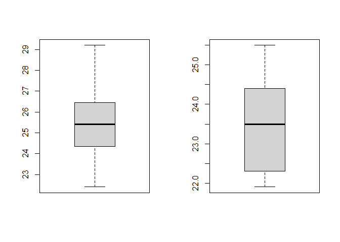
par(mfrow = c(1, 1)) # this returns the plot area for a single plot. You need to run this, otherwise future plots will continue to be plotted with 1 row and 2 columns (meaning two plots per figure)
As you can see, there are no outliers in the data.
One-way ANOVA
One-way ANOVA (Analysis of Variance) is a hypothesis test to determine whether the means from more than two populations or groups are equal or not.
As an example, suppose that four basketball teams took a random sample of players regarding how high each player can jump (in inches). μ1 = μ2 = μ3 = μ4 is the null hypothesis. The alternative hypothesis is at least one μ is statistically different from the rest.
We first input the data into an appropriate format (add to a code chunk in your RMarkdown file, and then send it to the command line).
# Create vector of jump heights (in inches)
height <- c(36, 42, 51, 32, 35, 38, 48, 50, 39, 38, 44, 46)
# Create vector of team names
team <- c(rep("T1",3), rep("T2",3), rep("T3", 3), rep("T4", 3))
# Merge
df <- data.frame(height, team)
# Visualize the data
print(df)
##    height team
## 1      36   T1
## 2      42   T1
## 3      51   T1
## 4      32   T2
## 5      35   T2
## 6      38   T2
## 7      48   T3
## 8      50   T3
## 9      39   T3
## 10     38   T4
## 11     44   T4
## 12     46   T4
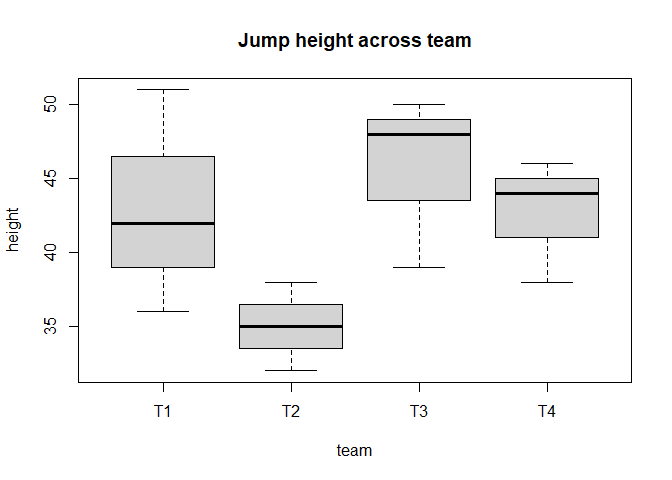
We can make a boxplot to visualize the data by team. Add the following to a code chunk in your RMarkdown file, and then send it to the command line:
# Box plot of jump height  for each team
boxplot(height ~ team, data = df, main = "Jump height across team")
The function aov() can be used for fitting ANOVA models. The general form is aov(response ~ factor, data = data_name), where response represents the response variable and factor the variable that separates the data into groups. Once the ANOVA model is fit, we use the summary() function to view the result, which is in a standard ANOVA table. Add the following to a code chunk in your RMarkdown file, and then send it to the command line:
# Fits the anova model
model <- aov(height ~ team, data = df)
# See results
summary(model)
##             Df Sum Sq Mean Sq F value Pr(>F)
## team         3  189.6   63.19   2.148  0.172
## Residuals    8  235.3   29.42
With a p-value of 0.172 (which is larger than 0.05), we fail to reject the null hypothesis. In other words, we do not have enough evidence to conclude that the mean jump height of any group is different from the other.
Assumptions
The ANOVA test makes three main assumtpions about the data:
-
The data in each group is normally distributed.
-
The variance of the data is the same across all groups.
-
Each observation is independent from another. In the same way as above, we cannot test but have to assume based on the way the data was collected.
To test if each group is normally distributed, you can again perform the Shapiro-Wilk test on each group.
# Performs shakiro-wilk test on each group to assess normality
shapiro.test(df$height[df$team == "T1"])
shapiro.test(df$height[df$team == "T2"])
shapiro.test(df$height[df$team == "T3"])
##
##  Shapiro-Wilk normality test
##
## data:  df$height[df$team == "T1"]
## W = 0.98684, p-value = 0.7804
##
##
##  Shapiro-Wilk normality test
##
## data:  df$height[df$team == "T2"]
## W = 1, p-value = 1
##
##
##  Shapiro-Wilk normality test
##
## data:  df$height[df$team == "T3"]
## W = 0.88107, p-value = 0.3275
All p-values are larger than 0.05, so we assume that the data from each team comes from a normal distribution. Instead of performing a Shapiro-Wilk test separately on each group, you could also test if the residuals of the model are normally distributed. To know more about how to do this, check this link.
To test if the variance is the same across groups, you can do a Bartlett test, which tests how probable is your data under a null hypothesis of equal variance across groups.
# Performs a Bartlett test to check for equality in variance
bartlett.test(height ~ team, data = df)
##
##  Bartlett test of homogeneity of variances
##
## data:  height by team
## Bartlett's K-squared = 1.4851, df = 3, p-value = 0.6857
Here, the p-value of 0.6857 is larger than 0.05, which tell us that we cannot reject the null hypothesis that the groups have similar variances.
A final note on testing assumptions: here, we have showed some simple ways to test assumptions of your tests. However, we recommend that you also familiarize yourself with visual ways to test assumptions, such as qqplots to check for normality. If you want a more detailed explanation of how to visually test assumptions (and about these tests overall), this is a great resource.
The R Markdown file
Your Markdown file now may now look like this:
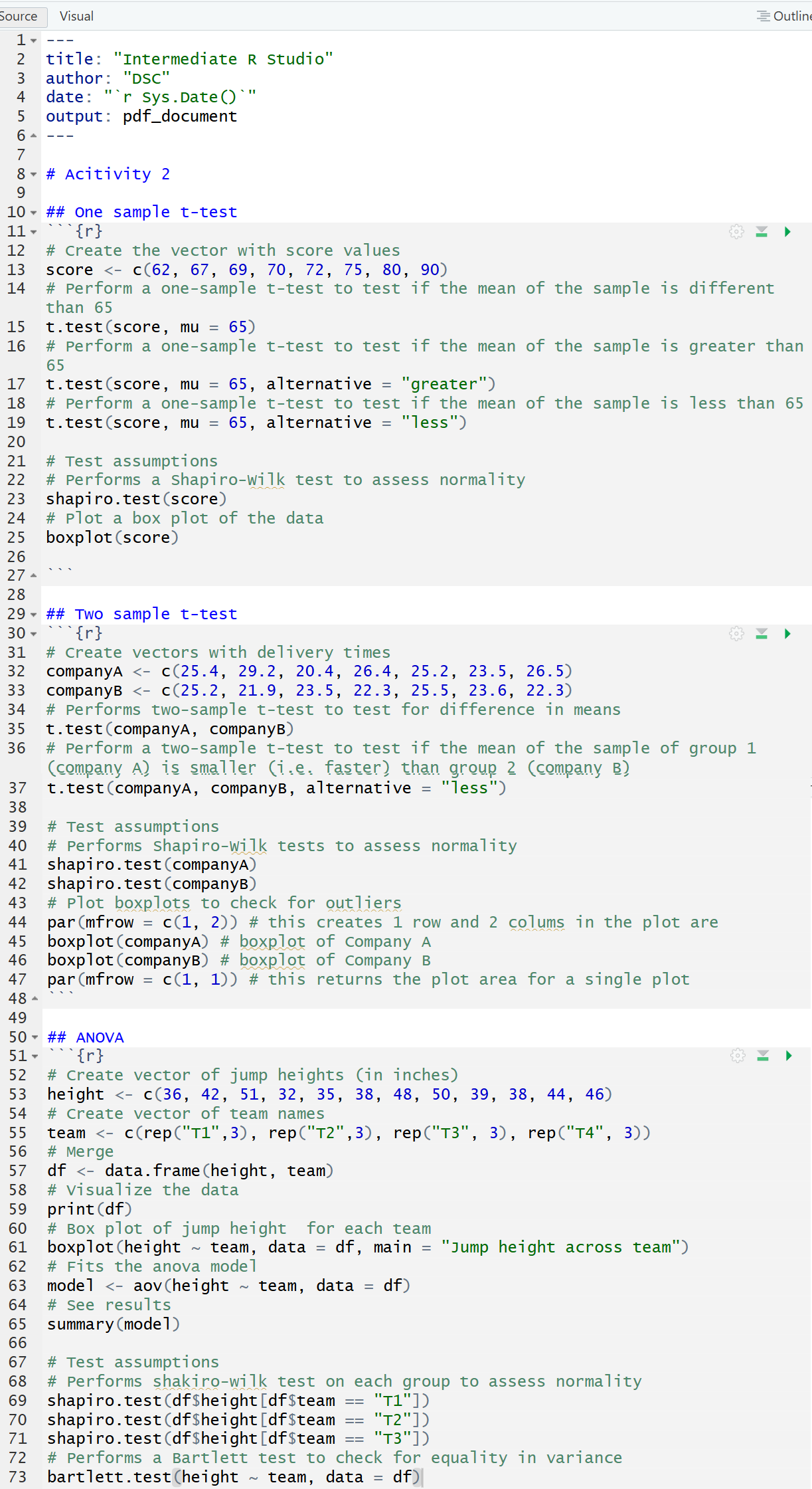
Click on the “Knit” buttom to knit your file into .pdf and then check the .pdf produced (by default, it is saved on the same folder as the .Rmd file) to see how R Markdown works.