Fundamental Excel Skills
If you and your group have any questions or get stuck as you work through this in-class exercise, please ask the instructor for assistance. Have fun!
- Open Excel, and open a Blank workbook.
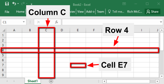
- Rows, columns, and cells defined:
- Columns are vertical. Eg. Column C.
- Rows are horizontal. Eg. Row 3.
- Cells are the intersection between a column and a row. Eg. Cell E7 (see image).
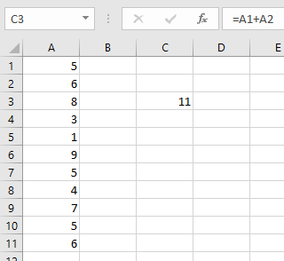
- Enter number 5 into cell A1 in your spreadsheet, and then press Enter on your keyboard.
- Enter the following numbers in Column A below the number 5 you just entered: 6, 8, 3, 1, 9, 5, 4, 7, 5, 6. We will use this list of numbers for the rest of this exercise.
- Basics operation on cells. Excel can perform basic mathematical operations with numbers stored in cells.
- Click on Cell C3, press the = sign, then use your mouse and click on A1, press the + sign, then click on Cell A2. Cell C3 should have the following in it: =A1+A2. Now press Enter on your keyboard, and Excel will add cells A1 and A2 together and display the number 11 in Cell C3.

- Click on or Select Cell C5, and then type in =A3-A4 Now press Enter on your keyboard, and Excel will display 5 in Cell C5 (8-3=5).

- Click on another cell and do the same thing to multiply two or more cells together using the * symbol to multiply.

- Click on another cell and do the same thing to divide two or more cells using the / symbol to divide.

- Click on Cell C3, press the = sign, then use your mouse and click on A1, press the + sign, then click on Cell A2. Cell C3 should have the following in it: =A1+A2. Now press Enter on your keyboard, and Excel will add cells A1 and A2 together and display the number 11 in Cell C3.
- Copying & pasting into ranges with the default Relative Cell Referencing. Instead of copying and pasting manually, you can drag values through the cells, and Excel will automatically copy and paste the content.
- In cell B1 type 5 and then press Enter. Click on B1, then select the green dot on the bottom right of the cell and drag it down to cell B11. You should now have a column of 5’s.
- Note: You can also use the “drag down” option to automatically fill sequential values. For example, type in 5 in cell B1 and 6 in cell B2. Then, select both cells B1 and B2, select the green dot on the bottom right of the cells and drag it down to cell B11. You should now have a column of sequential values (5, 6, 7, etc).
- Delete the data currently in column C, and make column B a column of 5’s again. Then, in cell C1, enter: =A1*B1 and press Enter. Click on C1, then select the green dot on the bottom right of the cell and drag it down to cell C11. You’ve just multiplied all the rows in columns A and B and put the result in column C!

- The above was possible due to Relative Cell Referencing, which adjusts the cell referenced based on its location. That is, when typing “A1*B1” in cell C1 above, Excel actually stores the information that you are multiplying cells one and two columns to the left of the current cell. When you dragged down the formula, it automatically adjusted the cell referenced. For example, if you click on cell C11, you will see that Excel adjusted the formula for “=A11*B11”.
- In cell B1 type 5 and then press Enter. Click on B1, then select the green dot on the bottom right of the cell and drag it down to cell B11. You should now have a column of 5’s.
-
Relative cell referencing is the default. You can avoid relative cell referencing, by using Absolute Cell Reference:

- Delete the contents of columns B and C except for the first row (cells B1 and C1).
- Double-click on cell C1, and then edit the formula to look like this: =A1*B$1. the Press Enter. The $ sign locks the reference to cell B1 always to row 1, even if you drag it down.
- Click on C1, select the green dot on the bottom right of the cell & drag it down to cell C11.
- Click on cell C11 and see that it reads =A11*B$1.
- For more information, read this short guide on cell referencing view this page. It will be useful when we work with functions such as XLOOKUP in Activity 3.
- Beyond knowing how to use relative and absolute cell referencing, it is good to know how to use dynamic formulas. Dynamic formulas will automatically perform the relative cell reference and drag down action for you.
- Delete the contents in columns B and C
- Type 1 in cell B1 and 2 in cell B2. Then, select both cells B1 and B2, select the green dot on the bottom right of the cells and drag it down to cell B11, making column B contain a sequential set of values from 1 to 11.
- In cell C1, type =A1:A11*B1:B11 (Instead of typing A1:A11 and B1:B11, you could also select these cells directly), then click enter
- You will see that Excel will automatically perform the multiplication of values A and B for each row, as if you had dragged the formula down using relative cell referencing.
- This not only saved you time, but also prevents mistakes from happening as no value in column C can be accidentally deleted or substituted (which could happen if using relative cell referencing)
-
OPTIONAL. but highly recommended: Check this short Youtube Video (1min) to learn about some useful keyboard shortcuts to navigate cells in Excel.
-
OPTIONAL: The Text to Columns tool can come in handy when you want to split a table of text (like on a web page) into multiple cells. If you’d like more information on converting text to columns, view this video
-
OPTIONAL: Sometimes you might want to visualize only sections of your data. You can do that using the filter button in Excel. If you’d like more details on filtering data in a range, view this video
- OPTIONAL: Data Cleaning using Find, Replace & Pivot Tables:
- Cleaning your data is an important process to make sure your dataset is correct before you start your analysis. At this stage, there are often common mistakes that you want to check for, and you can use the Find & Replace tool for that. If you’d like more details on finding or replacing data, view this video
- Sorting a column of data and then looking down it for misspellings can also help you detect mistakes. Here’s a quick explanation on how to sort data. Attention, when sorting, you want to make sure that Excel is taking into account all your data together, and not just sorting one column while leaving the others as they were, this might mix up your data. To avoid this, check these instructions
- For very large data sets, you can create a Pivot table - using the “group by” function - which can help you quickly identify misspelled words. We will cover Pivot Tables in the intermediate section of this workshop.
- For larger and more complex datasets, OpenRefine is a more powerful tool than Excel for cleaning data: OpenRefine is a free, open-source tool.
- Data Validation:
- One of the easiest ways to validate data is to use an input form with radio boxes or drop-down menus as you see in all online survey tools. Google Sheets has an excellent Forms tool that can be used to collect data you enter yourself or survey data from research participants. Google Forms, puts the data into Google Sheets, which can then be either analyzed in Google Sheets or exported to MS Excel. Here is more information about Google Forms
- If you’d like more information on data collections forms and validation in Excel, view please follow along with this video